Spinning Up: Part 1 Key Concepts inb RL
RL Spinning Up: Part 1 Key Concepts inb RL
Welcome to Spinning Up in Deep RL! — Spinning Up documentation
Introduction to RL
Part 1: Key Concepts in RL

Concepts:
- states and observations,
- action spaces,
- policies,
- trajectories,
- different formulations of return,
- the RL optimization problem,
- and value functions.
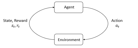
- The agent interacts with the environment, and takes actions($a$).
- Then the agent gets observations($o$), and takes actions again.
- While the agent takes actions, the environment changes, but may also change on its own,
Reward is the signal from the environment, the goal of the agent is to maximize its cumulated reward, called return.
States and observations
- $s$ has all the information of the world.
- $o$ is just a partial description of a state.
- Fully observed && Partially observed
Action space: all valid actions in the environment
- Discrete action spaces
- Continuous action spaces
Policies($\mu$): rules used to decide which actions to take, \[a_t = \mu(s_t).\]
Or stochastic: \[a_t \sim \pi(\cdot | s_t).\]
We often denote the parameters of policies by $\theta$, or $\phi$: \[\begin{cases} a_{t} =\mu _{\theta }( s_{t})\\ a_{t} =\pi _{\theta }( \cdot |s_{t}) \end{cases}\]
Two key computations on Stochastic Policies:
- Sampling actions from the policy.
- Computing log-likelihoods of actions, $\log \pi_\theta (a\mid s)$
This process is like training a classifier acting actions to get best log-likelihoods.
Log-likelihoods \[\log\pi_\theta(a|s) = log[P_\theta(s)]_a\]
Diagonal Gaussian Policies
- with mean vector $\mu$, and covariance $\Sigma$
- Diagonal gaussian distribution just has values on the diagonal, so it can be a vector.
- $o \xrightarrow{NN} \mu_{\theta }(s_t)$
Two ways of covariance:
- Stand alone parameters $\log\sigma$.
- Neuro network $s \xrightarrow{NN} \log \sigma_\theta( s)$
Sampling:
Given the mean action $\mu_\theta(s)$ and standard deviation $\sigma_\theta(s)$, and the vector $z$ of noise from spherical Gaussian ($z\sim \mathcal{N}(0, I)$): \[a=\mu_\theta(s)+\sigma_\theta(s) \odot z,\]
which $\odot$ denote the elementwise product of two vectors.
Log-likelihood of $k$-dim action $a$: \[\log \pi_\theta(a \mid s)=-\frac{1}{2}\left(\sum_{i=1}^k\left(\frac{\left(a_i-\mu_i\right)^2}{\sigma_i^2}+2 \log \sigma_i\right)+k \log 2 \pi\right)\]
Trajectories
A trajectory is a sequence of states: \[\tau=(s_0, a_0, s_1, a_1, ...),\]
which $s_0\sim\rho_0(\cdot)$, and $\rho_0$ is the start state distribution.
State transitions: $s_{t+1}=f(s_t, a_t)$, or stochastic $s_{t+1}\sim P(\cdot \mid s_t, a_t)$
Reward and return
We use $r_t$ as reward at $t$ time: \[r_t = R(s_t, a_t, s_{t+1})\simeq R(s_t,a_t)\simeq R(s_t)\]
Two kinds of return:
Finite-horizon undiscounted return \[R(\tau)=\sum_{t=0}^T r_t,\]
Infinite-horizon discounted return \[R(\tau)=\sum_{t=0}^\infty \gamma^t r_t,\]
Why use $\gamma^t$?
- intuitively appealing: cash now » cash later.
- math convenient: converge to a finite value.
RL Problem
Goal of RL: Agent actions -> policy -> max{expected return}
$T$-step trajectory: \[P(\tau \mid \pi)=\rho_0\left(s_0\right) \prod_{t=0}^{T-1} P\left(s_{t+1} \mid s_t, a_t\right) \pi\left(a_t \mid s_t\right)\]
The expected return: \[J(\pi)=\int_\tau P(\tau \mid \pi) R(\tau)=\underset{\tau \sim \pi}{\mathrm{E}}[R(\tau)]\]
The central optimization problem in \[\pi^*=\arg \max _\pi J(\pi)\]
Value Function
Value is the expected return if keeping on acting current policy.
- On-Policy Value Function: start at $s$, taking policy $\pi$
- On-Policy Action-Value Function: start at $s$, for any action $a$, taking policy $\pi$
- The Optimal Value Function: start at $s$, taking the optimal policy:
- The Optimal Action-Value Function: start at $s$, for any action $a$, taking the optimal policy:
Thus, we get: \[V^\pi(s)=\underset{a \sim \pi}{\mathrm{E}}\left[Q^\pi(s, a)\right], \\ V^*(s)=\max _a Q^*(s, a)\]
Optimal Q-Function and Action
The optimal action-value function $Q^*(s, a)$ is starting at $s$, for any action $a$, taking the optimal policy forever.
Thus, if we have $Q^*$, then we get: \[a^*(s)=\arg \max_a Q^*(s, a)\]
Bellman Equation
All equations follow the self-consistency equation: Bellman Equation:
The value of your starting point is the reward you expect to get from being there, plus the value of wherever you land next.
For on-policy value function: \[\begin{aligned} V^\pi(s) & =\underset{\substack{a, \sim \pi \\ s^{\prime} \sim P}}{\mathrm{E}}\left[r(s, a)+\gamma V^\pi\left(s^{\prime}\right)\right], \\ Q^\pi(s, a) & =\underset{s^{\prime} \sim P}{\mathrm{E}}\left[r(s, a)+\gamma \underset{a^{\prime} \sim \pi}{\mathrm{E}}\left[Q^\pi\left(s^{\prime}, a^{\prime}\right)\right]\right], \end{aligned}\]
where $s^{\prime} \sim P$ is shorthand for $s^{\prime} \sim P(\cdot \mid s, a)$, indicating that the next state $s^{\prime}$ is sampled from the environment’s transition rules; $a \sim \pi$ is shorthand for $a \sim \pi(\cdot \mid s)$; and $a^{\prime} \sim \pi$ is shorthand for $a^{\prime} \sim \pi\left(\cdot \mid s^{\prime}\right)$.
Then, for the optimal value functions: \[\begin{aligned} V^*(s) & =\max _a \underset{s^{\prime} \sim P}{\mathrm{E}}\left[r(s, a)+\gamma V^*\left(s^{\prime}\right)\right], \\ Q^*(s, a) & =\underset{s^{\prime} \sim P}{\mathrm{E}}\left[r(s, a)+\gamma \max _{a^{\prime}} Q^*\left(s^{\prime}, a^{\prime}\right)\right] . \end{aligned}\]
Advantage Functions
People want to know how much the action is better than other on average, using advantage functions: \[A^\pi(s,a) = Q^\pi(s,a) - V^\pi(s).\]
This describes in $s$, how taking $a$ is better than taking random $\pi( \cdot \mid s )$.
Formalism
Markov Decision Processes (MDPs). An MDP is a 5-tuple, $\left\langle S, A, R, P, \rho_0\right\rangle$, where
- $S$ is the set of all valid states,
- $A$ is the set of all valid actions,
- $R: S \times A \times S \rightarrow \mathbb{R}$ is the reward function, with $r_t=R\left(s_t, a_t, s_{t+1}\right)$,
- $P: S \times A \rightarrow \mathcal{P}(S)$ is the transition probability function, with $P\left(s^{\prime} \mid s, a\right)$ being the probability of transitioning into state $s^{\prime}$ if you start in state $s$ and take action $a$,
- and $\rho_0$ is the starting state distribution.
Understanding
\(V^\pi(s)=\underset{\tau \sim \pi}{\mathrm{E}}\left[R(\tau) \mid s_0=s\right]\)
- $\pi \overset{sample}{\longrightarrow} \tau$, for deep search
- \[Q^\pi(s_t,a)=\begin{cases}a \\V^\pi(s_{t+1})\end{cases}\]
\(V^\pi(s)=\underset{a \sim \pi}{\mathrm{E}}\left[Q^\pi(s, a)\right]\)
- $s_t \overset{a}{\longrightarrow} s_{t+1}$
- $V^\pi(s_t) \overset{a}{\rightarrow} Q^\pi(s_t, a)$
\(V^\pi(s) =\underset{\substack{a, \sim \pi \\ s^{\prime} \sim P}}{\mathrm{E}}\left[r(s, a)+\gamma V^\pi\left(s^{\prime}\right)\right],\)
- Backtracking + Recursion
- $s_t \rightarrow s_{t+1}$
- $s_{t}\overset{?}{\leftarrow} s_{t+1}$
- $V^\pi(s)=\underset{a \sim \pi}{\mathrm{E}}\left[Q^\pi(s, a)\right]$
- $Q^\pi-\mathrm{E}(Q^\pi)$