Spinning Up: Part 3: Intro to Policy Optimization
RL Spinning Up: Part 3 Intro to Policy Optimization
Welcome to Spinning Up in Deep RL! — Spinning Up documentation
Deriving the Simplest Policy Gradient
Optimize the policy by gradient ascent: \[\theta_{k+1}=\theta_k+\left.\alpha \nabla_\theta J\left(\pi_\theta\right)\right|_{\theta_k}\]
- Expression for policy gradient
- deriving the analytical gradient of policy performance
- forming a sample estimate of that expected value
Probability of a Trajectory. \[P(\tau \mid \theta)=\rho_0\left(s_0\right) \prod_{t=0}^T P\left(s_{t+1} \mid s_t, a_t\right) \pi_\theta\left(a_t \mid s_t\right)\]
The Log-Derivative Trick, we get: \[\nabla_\theta P(\tau \mid \theta)=P(\tau \mid \theta) \nabla_\theta \log P(\tau \mid \theta)\]
- $g(x)=\log f(x)$
- $\nabla g(x) = \nabla f(x)/f(x)$
- $\nabla f(x) = \nabla g(x) f(x)= \nabla \log (f(x)) f(x)$
Log-Probability of a Trajectory. The log-prob of a trajectory is just \[\log P(\tau \mid \theta)=\log \rho_0\left(s_0\right)+\sum_{t=0}^T\left(\log P\left(s_{t+1} \mid s_t, a_t\right)+\log \pi_\theta\left(a_t \mid s_t\right)\right) .\]
Gradients of Environment Functions. The environment has no dependence on $\theta$, so gradients of $\rho_0\left(s_0\right)$, $P\left(s_{t+1} \mid s_t, a_t\right)$, and $R(\tau)$ are zero.
Grad-Log-Prob of a Trajectory. The gradient of the log-prob of a trajectory is thus
Derivation for Basic Policy Gradient \[\begin{align} \nabla_\theta J(\pi_\theta) &= \nabla_\theta \mathbb{E}_{\tau \sim \pi_\theta} \left[ R(\tau) \right] && \text{} \\ &= \nabla_\theta \int_\tau P(\tau \mid \theta) R(\tau) \, d\tau && \text{Expand expectation} \\ &= \int_\tau \nabla_\theta P(\tau \mid \theta) R(\tau) \, d\tau && \text{Bring gradient under integral} \\ &= \int_\tau P(\tau \mid \theta) \nabla_\theta \log P(\tau \mid \theta) R(\tau) \, d\tau && \text{Log-derivative trick} \\ &= \mathbb{E}_{\tau \sim \pi_\theta} \left[ \nabla_\theta \log P(\tau \mid \theta) R(\tau) \right] && \text{Return to expectation form} \\ \therefore \nabla_\theta J(\pi_\theta) &= \mathbb{E}_{\tau \sim \pi_\theta} \left[ \sum_{t=0}^T \nabla_\theta \log \pi_\theta(a_t \mid s_t) R(\tau) \right] && \text{Expression for grad-log-prob} \end{align}\]
If we collect a set of trajectories $\mathcal{D}=\left{\tau_i\right}_{i=1, …, N}$ , the policy gradient can be estimated with \[\hat{g}=\frac{1}{\vert \mathcal{D} \vert} \sum_{\tau \in \mathcal{D}} \sum_{t=0}^T \nabla_\theta \log \pi_\theta\left(a_t \mid s_t\right) R(\tau)\]
where $\vert \mathcal{D}\vert$ is the number of trajectories in $\mathcal{D}$ (here, $N$ ).
Implementing the Simplest Policy Gradient
Expected Grad-Log-Prob Lemma
EGLP Lemma. Suppose that $P_{\theta}$ is a parameterized probability distribution over a random variable, $x$. Then: \[\underset{x \sim P_\theta}{\mathrm{E}}\left[\nabla_\theta \log P_\theta(x)\right]=0.\]
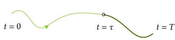
Don’t Let the Past Distract You
Policy gradient: \[\nabla_\theta J(\pi_\theta) = \underset{\tau \sim \tau_\theta}{\mathrm{E}} \left[ \sum_{t=0}^T \nabla_\theta \log \pi_\theta (a_t \mid s_t)R(\tau) \right].\]

- Agent should only reinforce actions on consequence: only rewards coming after.
So we only reinforced based on rewards obtained after: \[\nabla_\theta J\left(\pi_\theta\right)=\underset{\tau \sim \pi_\theta}{\mathrm{E}}\left[\sum_{t=0}^T \nabla_\theta \log \pi_\theta\left(a_t \mid s_t\right) {\color{green}\sum_{t^{\prime}=t}^T} R\left(s_{t^{\prime}}, a_{t^{\prime}}, s_{t^{\prime}+1}\right)\right] .\]
We’ll call this form the “reward-to-go policy gradient,” \[\hat{R}_t \doteq \sum_{t^{\prime}=t}^T R\left(s_{t^{\prime}}, a_{t^{\prime}}, s_{t^{\prime}+1}\right)\]
Implementing Reward-to-Go Policy Gradient
Baselines in Policy Gradients
Consequence of the EGLP lemma is: for any function $b$ which depends on state, \[\underset{a_t \sim \pi_\theta}{\mathrm{E}}\left[\nabla_\theta \log \pi_\theta\left(a_t \mid s_t\right) b\left(s_t\right)\right]=0\]
This allows us to add or subtract, without changing it in expectation: \[\nabla_\theta J\left(\pi_\theta\right)=\underset{\tau \sim \pi_\theta}{\mathrm{E}}\left[\sum_{t=0}^T \nabla_\theta \log \pi_\theta\left(a_t \mid s_t\right)\left(\sum_{t^{\prime}=t}^T R\left(s_{t^{\prime}}, a_{t^{\prime}}, s_{t^{\prime}+1}\right)- {\color{green}b\left(s_t\right)}\right)\right] .\]
Function $b$ called baseline.
The normal baseline is $V^\pi(s_t)$, as average return under policy $\pi$ for rest of time.
Empirically, $b(s_t)=V^\pi(s_t)$ has the desirable effect on reducing variance, making the learning more stable: If the agent gets its expectation, it feel neutral about it.
In practice, we use the value network $V_\phi (s_t)$ to approximate $V^\pi(s_t)$.
The simplest way of learning $V_\phi (s_t)$ is, \[\phi_k=\arg \min _\phi \underset{s_t, \hat{R}_t \sim \pi_k}{\mathrm{E}}\left[\left(V_\phi\left(s_t\right)-\hat{R}_t\right)^2\right]\]
where $\pi_k$ is the policy at epoch $k$, from $\phi_{k-1}$ by one or more gradient descent.
Thus, we get general formation: \[\nabla_\theta J\left(\pi_\theta\right)= \underset{\tau \sim \pi_\theta}{\mathrm{E}} \left[ \sum_{t=0}^T \nabla_\theta \log \pi_\theta\left(a_t \mid s_t\right) {\color{green}\Phi_t} \right] .\]
where $\Phi_t$ could be: \[\Phi_t = \begin{cases} R(\tau) \\ \sum\limits_{t' = t}^{T} \displaystyle R(s_t^{\prime}, a_t^{\prime}, s_{t+1}^{\prime}) \\ \sum\limits_{t' = t}^{T} \displaystyle R\left(s_t^{\prime}, a_t^{\prime}, s_{t+1}^{\prime}\right) - b\left(s_t\right) \end{cases}\]
On-Policy Action-Value Function \[\Phi_t=Q^{\pi_\theta}(s_t, a_t)\]
The Advantage Function ($A^{\pi_\theta}(s_t,a_t) = Q^{\pi_\theta}(s_t,a_t) - V^{\pi_\theta}(s_t)$) \[\Phi_t = A^{\pi_\theta}(s_t,a_t)\]
- this equivalent to $\Phi_t=Q^{\pi_\theta}(s_t, a_t)$ and using $b(s_t)=V^\pi(s_t)$.
Understanding
| Method | Expectation | Variance |
|---|---|---|
| Model (Neuron Network) | Bad | Good |
| MC (Monte Carlo Estimation) | Good | Bad |
GAE: find proper method to estimate average value function $V^\pi$:
| Distance | Expectation | Variance |
|---|---|---|
| Too short | Bad | Good |
| Too long | Good | Bad |
Adding $\lambda$ to balance Expectation and Variance.
- \[A_t^{\lambda} = \sum_{l=0}^{\infty} (\gamma\lambda)^l \delta_{t+l}\]